Microsoft Excel : Formula Result not showing

Hi,
Lets get known to a common Microsoft Excel issue.

Issue/Problem

Last day, I was working with a file in my office. That file was in Microsoft Excel format and I have to analyze data. When placing some formula, I noticed, excel is not calculating formula.
Lets be clear with following screenshot.

I tried many thing, Converted File to older format, newer format, opened and closed in other system and many other tricks but no one worked.

Actual Cause

Then suddenly I show the Format of the textbox where formula is placed. That is of kind Text and was the actually reason for not calculating formula. Microsoft Excel treats everything as normal Text string while placed or formatted as Text.

Solution

I have following two simple steps and Results are back.
Step 1: Changed formatting of Cell to Number which is of course my data type for the result. Lets have look at below screen to be more clear.

Step 2: Clicked in Cell to go to edit mode and pressed Enter key without any modification as formula was correct. Have a look at this screen to confirm.

Problem solved.

If you find my posts helpful, do not forget to share on social network or with your friends. Suggestions and feedback are awaited and always welcome.

+John Bhatt 

Read More

Problem Opening Office Documents

Hi,
Today I want to tell you about a common problem that you must have faced if you are still using MS Office 2003. When you tried to open the document created by Ms Office 2007, 2010 or 2013 by default this is in different extension and shows error while opening in lower version. To escape from this problem you either have to uninstall your MS Office package and upgrade to higher version (at least MS office 2007) or Ask the author of file to send a compatible file in Office 1997-2003 version.

But here is a best way that you can try without any cost and without any request.To open all types of Office Documents that are of created with higher versions of MS Office, you can download Office Converter. Microsoft has published it as Compatibility Pack for 2007 Office System.

You may follow the link to downnload Microsoft Office Document Converter.
Steps:

• Save Downloaded file to disk.
• When download completes, run the executable file.
• Proceed to installation.
• When complete, reboot your system.

This will install all rendering engine in your Office 2003 and you can open your existing files as well as files with newer version.

+John Bhatt

Read More

Microsoft Excel : Text Functions Part -3

Hi,

In previous post we have talked about some of the Text functions in detail. We will continue this post from where we left.

If you have not read previous posts, this post might be some confusing to you. I will request you to read these posts before proceeding.

Text Functions in Microsoft Excel Part -1

Text Functions in Microsoft Excel Part –2

Directly moving ahead to function details and their use.

9. FIXED()

Introduction: FIXED function Rounds a number to the specified number of decimals, formats the number in decimal format using a period and commas, and returns the result as text.
Using Method: This function takes minimum of one and maximum of 3 parameters. First one is Number, this can be any number value or reference to a cell. Second is the decimals , for rounding. Last one is a Boolean option for keeping period separator or not.

=FIXED(139493.4532,2) or =FIXED(A1,-1,TRUE)

Example:

NOTE: Difference between ROUND function and FIXED function is, FIXED converts number to text after rounding but ROUND keep number to number after rounding.

10. LEFT()

Introduction: LEFT function returns specified number of characters from start based in start number (length) in a string.

Using Method: This function takes two parameters. First one is text to be searched, this can be simple string value or reference to a cell. Second is the number of characters to start.
=LEFT("Hello World",6) or =LEFT(A1,6)

Example:

11. LEN()

Introduction: LEN function returns number of characters in a string. In simple words, it returns the length of a string.

Using Method: This function takes single parameter and that is of type string or reference to a cell.

=LEN(“Hello World”) or =LEN(A1)

Example:

 

12. LOWER()

Introduction: LOWER function converts all characters in a string to lower case.
Using Method: This function takes a single parameter and that is of type string or reference to a cell.

=LOWER(“Hello World”) or =LOWER(A1)

Example:

 

13. MID()

Introduction: MID function returns the middle characters from a string specified by start number and length.
Using Method: This function takes three parameters. One is text which is required, another is Start number to search from and another is number of character to show or length to be picked.
=MID(“John is from Nepal”,9,10) or =MID(A1,9,10)

Example:

 

14. PROPER()

Introduction: PROPER function converts all characters and words to Title case as per English Grammar. Means all the beginning character of all words are in capital letter and other are in small letter regardless of their typography.
Using Method: This function takes a single parameter and that is text string or reference to cell .

=PROPER(“this is going to BE CHANGED in title”) or =PROPER(A1)

Example:

 

15. REPLACE()

Introduction: REPLACE function replaces a part of string with specified string.
Using Method: This function takes four parameters, First one is text to be replaced, then starting number of character where replace to be started, then number of character to replace (length), and final one is new text.
=REPLACE(A1,6,3,”was ”) or =REPLACE(A1,6,3,C1)

Example:

 

16. RIGHT()

Introduction: RIGHT function does the exactly same work as LEFT do but from opposite index. This returns the text from end of an string based on the length passed by user.
Using Method: This function takes two parameters and both are required. First one is string or reference to cell containing text and another is number of character to be shown.
=RIGHT(“The last five words”,5) or =RIGHT(A1,5)

Example:

  

I will be back with remaining text function in another post. Thanks for reading.

You can provide feedback using comments or contact page.

John Bhatt

Read More

Text Function : Microsoft Excel Part-2

Hi,

Lets come back to Excel series. We have previously talked about text functions in Excel. Before proceeding to detailed description and use of these functions, I would recommend you all to read previous part of this post at Text Functions in Microsoft Excel - Part 1.

1. BAHTTEXT()

Introduction: BAHT is the currency name of Thailand. This function simply convert the number to BAHT text and adds a sign also. But in Thai Text. In simple word, this function converts number to currency in Thai language.

Using Method: This function simply takes a single parameter. A number and writes BAHT amount in words.

=BAHTTEXT(1000) or =BAHTTEXT(A1)

Example: 

2. CHAR()

Introduction: CHAR function is derived from word character. As simply name suggests, this function returns the character of your input number based in your computer setting. This takes value from 0-255 and returns all the character set based in your value.

Using Method: This function takes single parameter and that is integer from 0-255.

=CHAR(48)

Example: Suppose ASCII value for 0 (number zero) is 48.

3. CLEAN()

Introduction: CLEAN function simply removes the non-printable character from your supplied string. 

Using Method: This function takes single parameter and that is of any kind of value in cell.

=CLEAN(A1) or =CLEAN(CHAR(17)&"This is actual Printable Text."&CHAR(17))

Example:

4. CODE()

Introduction: CODE function works just opposite to CHAR function. This returns the character code of your system as input character. 

Using Method: This function takes single paramater and of type Character as input. 

=CODE("A") or =CODE(A1)

Example:

5. CONCATENATE()

Introduction: CONCATENATE function joins multiple text string into one single String. This works with multiple cells.

Using Method: This function can take multiple inputs of different types separated by comma (,).
=CONCATENATE(A1,A2,A3)

Example:

6. DOLLAR()

Introduction: DOLLAR function converts your number to currency format as per your system locale setting. If you are using United States as your location, then this function will put a dollar sign and comma separator. If you are in India, this will put a Rupees sign as per your system and write as currency.
Using Method: This function takes two parameter, one is value and other is decimal. Then this will convert your number to currency text with decimals as your choice.
=DOLLAR(100,2) or =DOLLAR(A1,2)
Example:

7. EXACT()

Introduction: EXACT function compares two strings and returns Boolean value, True or False. This is case sensitive. If two strings are exactly same, this function returns TRUE and if any of character is different, then FALSE.
Using Method: This function takes two parameters and both in String format from different cells.
=EXACT(A1,B1) or =EXACT("Google","GOOGLE")
Example:

8. FIND()

Introduction: FIND function returns the position of search string in another string. This is case sensitive. 

Using Method: This function takes minimum of two and maximum of 3 parameters. First one is Find text, this can be simple string value or reference to a cell. Second is the Within text, string where to be searched. Last one is Start number, starting position from where to search. This is optional field.

=FIND("Help",A1) or =FIND(A1,B1,2) 

Example: 

Keep reading. I will be writing about remaining function on later posts. Till then keep sharing your knowledge and feedback.

+John Bhatt 

Read More

Text Functions : Microsoft Excel Part-1

Hi,

After some gap, I am back with Excel Tutorials . Lets learn Microsoft Excel in depth and work with functions. In this post, I am going to discuss all of the text functions with examples.

Function

Some of the best and one line definitions of Function are as below.

• A function is a block of code that performs a calculation and returns a value.
• We define a function as a special type of binary relation.

In short, function is a piece of code that is programmed to perform specific task. There are also some functions in Microsoft excel which can be easily implemented to get better and correct output in timely manner. The most useful and important feature of Microsoft Excel function is, they update their value automatically if any of the parameter (cell value) changed. We need not to change or update the cell which contain formula. Even we can protect the cell which contain formula so that, no one can alter the formula in shared document. Functions in Excel are divided in many category according to their use and working nature. Some of them are Text, Date & Time, Logical, Maths & Trigonometry, Engineering etc.

Text Functions

We will be talking about text functions in this post.
Why we call these functions text function?

Clear, they work with text, they can manipulate text cells, they can process normal text. 

The complete list of all text functions is as below. The new functions are added as part of user requirement and improvement in newer version of Microsoft Office.This list is taken from Microsoft Office 2003, so all later versions of Microsoft Excel (2007, 2010, 2013) will work and procedure will be same for all.

1. BAHTTEXT()
2. CHAR()
3. CLEAN()
4. CODE()
5. CONCATENATE()
6. DOLLAR()
7. EXACT()
8. FIND()
9. FIXED()
10. LEFT()
11. LEN()
12. LOWER()
13. MID()
14. PROPER()
15. REPLACE()
16. RIGHT()
17. SEARCH()
18. SUBSTITUTE()
19. T()
20. TEXT()
21. TRIM()
22. UPPER()
23. VALUE()
    Functions added in Microsoft Office 2013.
24. NUMBERVALUE()
25. UNICHAR()
26. UNICODE()

I will be discussing the use of these function in detail on next post. Till then keep digging.

Do not forget to share if you find this post helpful. If you have any comment, please leave and let us know.
John Bhatt

Read More

Keyboard Shortcuts in Microsoft Excel 2003

Hi,

Lets have a look at some keyboard Shortcuts for Microsoft Excel.

Table of keyboard combinations

SN	Key	Action	Alternate
1	Ctrl+A	Select All
2	Ctrl+B	Bold
3	Ctrl+C	Copy
4	Ctrl+D	Fill Down
5	Ctrl+F	Find
6	Ctrl+F	Goto
7	Ctrl+H	Replace
8	Ctrl+I	Ralice
9	Ctrl+K	Insert Hyper Link
10	Ctrl+N	New Workbook
11	Ctrl+O	Open
12	Ctrl+P	Print
13	Ctrl+R	Fill Right
14	Ctrl+S	Save
15	Ctrl+U	Under Line
16	Ctrl+V	Paste
17	Ctrl+W	Close	File,Clse
18	Ctrl+X	Cut	Edit,Cut
19	Ctrl+Y	Repeat	Edit,Repeat
20	Ctrl+Z	Undo	Edit,Undo
21	F1	Help	Help,Contents and Index
22	F2	Edit	None
23	F3	Paste Name	Insert,Name,Past
24	F4	Repeat test action	Edit,Repeat,Works while not in Edit mode
25	F4	White typing a formula, Switch between absotule/reletave rels	None
26	F5	Goto	Edit,Goto
27	F6	Next pane	None
28	F7	Spell check	Tools,Speling
29	F8	Extent mode	None
30	F9	Recaicutate all work book	Tools,Options,Calucation,Cale,Now
31	F10	Active Member	N/A
32	F11	New chart	Insert, Chart
33	F12	Save As	File,Save As
34	Ctrl+ :	Insert Cument Time	None
35	Ctrl+ ;	Insert Current Date	None
36	Cttrl+ "	Copy Value form Cell Above	Edit,Pest Special,Value
37	Ctrl+	Copy Formula form Cell Above	Edit,Copy
38	Shift	Hold down sift for additinaol in Excel's me	None
39	Shiftt+F1	What's This?	Help,What's This?
40	Shift+F2	Edit Cell Comment	Insert, Edit,Comments
41	Shift+F3	Pest function Into formulas	Insert, Function
42	Shift+F4	Find Next	Edit,Next,Find Next
43	Shift+F5	Find	Edit,Next,Find Next
44	Shift+F6	Previous pen	None
45	Shift+F8	Add to selection	None
46	Shift+F9	Calculete active worksheet	Calc Sheet
47	Shift+F10	Display shortcut menu	None
48	Shift+F11	New  worksheet	Insert, Worksheet
49	Shift+F12	Save	File,Save
50	Ctrl+F3	Define Name	Insert Names Define
51	Ctrl+F4	Close	File Close
52	Ctrl+F5	XL Restore window Size	Restore
53	Ctrl+F6	Next workbook window	Window,….
54	Shift +Ctrl+F6	Previous workbook window	Window,….
55	Ctrl+F7	Move window	XL,Move
56	Ctrl+F8	Resize window	XL,Size
57	Ctrl+F9	Minimize workbook	XL,Minimize
58	ctrl+F10	Maximize or Restore window	Xl,Maximize
59	Ctrl+F11	Insert 4.0 Micro Sheet	None Excel 97
60	Ctrl+F12	File open	File,Open
61	Alt+F1	Insert chart	Insert, Chart….
62	Alt+F2	Save As	File Save As
63	Alt+F4	Exit	File,Exit
64	Alt+F8	Micro diloge box	Tools,Micro,Microsins in year Excel 97 Tools,Macros - in earlier version
65	Alt+F11	Visual BasicEditor	Tools,Micro,Bisual Basic Editor
66	Ctrl+Shift+F3	Creat name by presing names  of row and column tables	Insert,Name,Create
67	Ctrl+Shift+F6	Previous window	Window
68	Ctrl+Shift+F12	Print	File,Print
69	Alt+Shift+F1	New worksheet	Insert,Worksheet
70	Alt+Shift+F2	Save	File,Save
71	Alt+=	Auto sum	No direct equivalent
72	Alt+	Toggle value/Formula display	Tool,Options,View,Formulas
73	Ctrl+Shift+A	Insert argument names Into formula	No direct equivalent
74	Alt+Down arrow	Display auto Complete list	None
75	Alt+"	Formula style dialog box	Formet,Style
76	Ctrl+Shift+~	General formet	Format, Sells, Number, Category ,General
77	Ctrl+Shift+!	Comma format	Format, Sells, Number, Category,Number
78	Ctrl+Shift+@	Time Formet	Format, Sells, Number, Category,Time
79	Ctrl+Shift+#	Date formet	Format, Sells, Number, Category,Date
80	Ctrl+Shift+$	Currency formet	Format, Sells, Number, Category,Currency,
81	Ctrl+Shift+%	Persent forment	Format, Sells, Number, Category,Persentage
82	Ctrl+Shift+^	Exponential formet	Format, Sells, Number, Category
83	Ctrl+Shift+&	Place autline border around selected cell	Formet,Cells,Border
84	Ctrl+Shift+_	Remove outlion border	Formet,Cells,Border
85	Ctrl+Shift+	Select current region	Edit,Goto,Special,Current Region
86	Ctrl++	Insert	Insert,(Ros,columns,or Cells)Depends on selection
87	Ctrl+-	Delete	Delete,(Ros,columns,or Cells)Depends on selection
88	Ctrl+1	Formet cell dilog box	Formet,Cells,Border
89	Ctrl+2	Bold	Formet,Cells,Font,Font style,Bold
90	Ctrl+3	Italic	Formet,Cells,Font,Font style,Italic
91	Ctrl+4	Under Line	Formet,Cells,Font,Font style,Underlion
92	Ctrl+5	Strikethrow	Formet,Cells,Font,Effects,Strikethrough
93	Ctrl+6	Show / Hide object	Tool,Options,View Objects,Show All/Hide
94	Ctrl+7	Show / Hide Standerd toolbar	View,Toolbar,Standard
95	Ctrl+8	Toggle outline symbols	None
96	Ctrl+9	Hide row	Formet,Row,Hide
97	Ctrl+0	Hide columns	Formet,Columns,Hide
98	Ctrl+Shift+(	Unhide row	Formet,Row,Underlion
99	Ctrl+Shift+)	Unhide columns	Formet,Columns,Underline
100	Alt or F10	Activet the menu	None
101	Ctrl+Tab	In toolbar : Next toolbsr	None
102	Shift+Ctrl+Tab	In toolbar : Privous toolbar	None
103	Ctrl+Tab	In a workbook : Active next workbook	None

Thanks to +Suresh kumar Awasthi for this collection. If you enjoyed and find this helpful, share this article or leave a feedback.

+John Bhatt 

Read More

Printing Header Rows (titles) in all pages of Microsoft Excel

Hi,

Once again, continuing Microsoft Excel series, I am going to tell you one more useful trick if you are working in office and use Excel for your work.

Introduction

You need to print data that is feeded in  Excel several times, but when data is larger, more than a page at printout, you need to print headers in top of the page. Or you need to print Column fixed in your printout. Earlier we have learnt how to fix columns in excel sheet and rows in excel sheet in previous posts.
Take a look at screenshots below, While we are looking in Print Preview, first page is showing header information in top but while in next page, there is no information, It is hard to know which column is it,

Procedure

Lets move to process directly without loosing time. Look at file we are working with.

1. Click on Page Layout tab.
2. Click on Print Titles command.
3. You will get Page Setup dialogue box open with Sheet tab.
   
    
4. Now Enter the Row numbers followed by Dollar sign ($) in Rows to repeat at top box, you can select using link button in box.
   
5. Click OK to apply settings.

Now look at the Print Preview once again.

Ok, its what you required.
Thanks for reading. If you find this post useful, do share and provide feedback.
+John Bhatt 

Read More

Fix Rows & Columns Simultaneously in Microsoft Excel

Hi,

Once again, moving ahead on Microsoft Excel series, We will learn another trick here. In previous posts, we have learnt how to fix one or more rows at same time and how to fix one or more columns at same time so that we can feel comfort with our data.
Now, it is time to fix row and columns simultaneously
Lets have a loot at the previous file we have created for demonstration. Vehicle Daily Status sheet.

We want here to fix the column A to E and rows 1,2 and 3. So that wherever we are on sheet, we know what field it is?
Lets move to process without loosing any time.

1. Click the Intersection point (cell) of rows and column you want to fix. 
2. Click on View Tab.
3. Click on Freeze Panes.
4. Click on Freeze Panes. 
   

You are done. Your output must be similar to this.

Have a look at Column Names and Row numbers I have highlighted in above snapshot.

If you have any questions or suggestions, drop a comment here. Do not forget to share if you found this helpful.

+John Bhatt 

Read More

Fix one or more Column in Microsoft Excel

Hi,
We will continue Microsoft Excel tutorials series. In last post in this topic, I have discussed about Fixing Headers in Microsoft Excel. We have learn how to fix one or more rows at same position while scrolling all data values in worksheet. If you have missed that read that post first.

Today, We will learn to Fix one or more columns which might be headers. The requirement is much similar like the previous scene, so I don't write more intro and requirement here.
Lets see, what we got first.

In above sheet, this is a sample format for Vehicle Tracking System on daily basis. Fist five columns are SN, Vehicle Number, Body Type of Vehicle, Driver Name and his mobile number which are important and we want them to fix at their position. Then we created Daily Status fields with simple two columns, one is Status and another is Location for that day. We expect that user will feed once a day and proceed ahead. But, in case you have lots of vehicles, suppose 200 or more and you are tracking for the day 28 or 29, what will be the scene at that time.
Just as we did in previous post, we will fix these Column fixed values and hide remaining data as we scroll to next date.

Process

If you have to fix, only on Column, there is a simple option provided in Microsoft Excel. In the View tab, there is Freeze Panes command, once you click on this, you will get option to Freeze First Column. That will do the job.
But, if you have more than one column to Fix. Follow these steps.

1. Click and select entire Column next to the Required Area. In above scene, I will select Column F.
2. Click on View Tab.
3. Click on Freeze Panes command.
4. Click on Freeze Panes option.
   
   
   

You have done it. Lets see the output.

If you find these posts helpful or any mistakes, you can thank or notify. Just drop a comment or leave a mail.

+John Bhatt 

Read More

Fix one or more Rows (Header) in Microsoft Excel

Hi,

Lets work with excel some more. After long back, I am going to continue my Excel series. Today we will learn about a very useful feature of Microsoft Excel.

Suppose we have headers in top row or 2nd or third row and lots of data. Suppose a thousand records or more. This generally happens at offices, schools and various workstations. We need to scroll down the page to view records but while it is large, we get confused with data, It is confusing that what is field header (i.e. What is data).

Lets be clear with below small example.

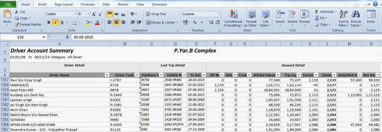
If above excel sheet. I have maintained ledger balance of Drivers of my company. This file has 2855 Rows (your file might have more or less).

While I have to view other records, I have to scroll the page. This will look like this snapshot.

What data is in column F, or G or H. If I do not remember, we have to scroll back and view headers and then come back to last position. To overcome this problem, Microsoft Excel has built-in feature called Freeze Rows or Panes. In this post, we will learn how to fix a Top row or more rows at same time.
If you are using Excel 2007, 2010 and 2013 the method is similar.

Lets go to process.

1. If Top row of your sheet is header, you need not to do anything, But if you have headers in second or third row, Select entire row below from header row by clicking in Row name..
2. Click on View Tab on Office Ribbon.
3. Click on Freeze Top Row if header in First row or Freeze Panes if header in second or third row. 

Now look at this. How it looked after scrolling down.

One thing most important about this feature. Your settings are saved within file. Means if you share file with other via email or other sharing tools, your settings remains same even if Microsoft Office version changes or system varies.

All the Best. If you found if helpful, do not forget to post a thank or +1 on Google.
+John Bhatt 

Read More

Microsoft Excel 2003 : File Menu and Its Commands-2

Hi,

I am back with Remaining part of Excel's File Menu and Commands.





As you remember, in previous post, we have talked about File Menu Commands upto Web Page Preview.
http://www.prithviraj.com.np/2012/06/microsoft-excel-2003-file-menu-and-its.html

Lets start with remaining commands.

11. Page Setup :

When you click this option Page Setup dialogue box appears from which you can adjust document margins, paper size, orientation, header footer, sheet, etc. This is one of the important option for printing document.

    12. Print Area :

This command sets the print area of current worksheet. You can choose which cell range should be printed in paper. You can also clear print area that you previously set. To Set a Print Area, choose range of cells by selecting, then click on File menu, choose Print Area option and finally choose Set Print Area option. To Remove a Print Area click on File menu, go to Print Area and choose Clear Print Area option.

   13. Print Preview :

This option shows how the document will appear after printing in paper. This is very important task before printing any document to save Paper and money. If any improvement needed you have to adjust document margins and other properties from Page Setup option. 

   14. Print (Ctrl+P) : 

This command sends instruction to attached printer that is configured with system. You have options to choose Printer, Page Range, Number of Copies, etc. Shortcut key for this command is CTRL+P.

   15. Send To :

If you want to send your excel workbook to other people via e-Mail you have following options to send the file. This command has following sub-menu:  

1. Mail Recipient
2. Mail Recipient (For Review)
3. Mail Recipient (As Attachment)
4. Routing Recipient
5. Exchange Folder
6. Online Meeting participant
7. Recipient using Internet Fax-Service

   16. Properties : 

This command shows you Document Properties dialogue box to edit or change properties of document such as Title, Subject, Author, Company, Keywords, and other values which are very important to determine the documents property value which will creates Identity of file.

17. Exit : 

This command terminates MS-Excel. This is alternative of ALT+F4 key. You can also quit application from Title Bar or Task bar also. If the document is not saved yet, MS-Word prompts you to save document and shows Save As dialogue box if chosen Yes from prompt and terminates after saving, if chosen No, terminates immediately and if chosen Cancel MS-Excel remains opened. 

Keep reading, for more Tutorials and Articles subscribe. 

All the Best. 

+John Bhatt 

Read More