Happy New Year 2014

Hi,

Wishing you and your family a very very happy and prosperous new year 2014.

+John Bhatt 

Read More

Keyboard Shortcuts in Microsoft Excel 2003

Hi,

Lets have a look at some keyboard Shortcuts for Microsoft Excel.

Table of keyboard combinations

SN	Key	Action	Alternate
1	Ctrl+A	Select All
2	Ctrl+B	Bold
3	Ctrl+C	Copy
4	Ctrl+D	Fill Down
5	Ctrl+F	Find
6	Ctrl+F	Goto
7	Ctrl+H	Replace
8	Ctrl+I	Ralice
9	Ctrl+K	Insert Hyper Link
10	Ctrl+N	New Workbook
11	Ctrl+O	Open
12	Ctrl+P	Print
13	Ctrl+R	Fill Right
14	Ctrl+S	Save
15	Ctrl+U	Under Line
16	Ctrl+V	Paste
17	Ctrl+W	Close	File,Clse
18	Ctrl+X	Cut	Edit,Cut
19	Ctrl+Y	Repeat	Edit,Repeat
20	Ctrl+Z	Undo	Edit,Undo
21	F1	Help	Help,Contents and Index
22	F2	Edit	None
23	F3	Paste Name	Insert,Name,Past
24	F4	Repeat test action	Edit,Repeat,Works while not in Edit mode
25	F4	White typing a formula, Switch between absotule/reletave rels	None
26	F5	Goto	Edit,Goto
27	F6	Next pane	None
28	F7	Spell check	Tools,Speling
29	F8	Extent mode	None
30	F9	Recaicutate all work book	Tools,Options,Calucation,Cale,Now
31	F10	Active Member	N/A
32	F11	New chart	Insert, Chart
33	F12	Save As	File,Save As
34	Ctrl+ :	Insert Cument Time	None
35	Ctrl+ ;	Insert Current Date	None
36	Cttrl+ "	Copy Value form Cell Above	Edit,Pest Special,Value
37	Ctrl+	Copy Formula form Cell Above	Edit,Copy
38	Shift	Hold down sift for additinaol in Excel's me	None
39	Shiftt+F1	What's This?	Help,What's This?
40	Shift+F2	Edit Cell Comment	Insert, Edit,Comments
41	Shift+F3	Pest function Into formulas	Insert, Function
42	Shift+F4	Find Next	Edit,Next,Find Next
43	Shift+F5	Find	Edit,Next,Find Next
44	Shift+F6	Previous pen	None
45	Shift+F8	Add to selection	None
46	Shift+F9	Calculete active worksheet	Calc Sheet
47	Shift+F10	Display shortcut menu	None
48	Shift+F11	New  worksheet	Insert, Worksheet
49	Shift+F12	Save	File,Save
50	Ctrl+F3	Define Name	Insert Names Define
51	Ctrl+F4	Close	File Close
52	Ctrl+F5	XL Restore window Size	Restore
53	Ctrl+F6	Next workbook window	Window,….
54	Shift +Ctrl+F6	Previous workbook window	Window,….
55	Ctrl+F7	Move window	XL,Move
56	Ctrl+F8	Resize window	XL,Size
57	Ctrl+F9	Minimize workbook	XL,Minimize
58	ctrl+F10	Maximize or Restore window	Xl,Maximize
59	Ctrl+F11	Insert 4.0 Micro Sheet	None Excel 97
60	Ctrl+F12	File open	File,Open
61	Alt+F1	Insert chart	Insert, Chart….
62	Alt+F2	Save As	File Save As
63	Alt+F4	Exit	File,Exit
64	Alt+F8	Micro diloge box	Tools,Micro,Microsins in year Excel 97 Tools,Macros - in earlier version
65	Alt+F11	Visual BasicEditor	Tools,Micro,Bisual Basic Editor
66	Ctrl+Shift+F3	Creat name by presing names  of row and column tables	Insert,Name,Create
67	Ctrl+Shift+F6	Previous window	Window
68	Ctrl+Shift+F12	Print	File,Print
69	Alt+Shift+F1	New worksheet	Insert,Worksheet
70	Alt+Shift+F2	Save	File,Save
71	Alt+=	Auto sum	No direct equivalent
72	Alt+	Toggle value/Formula display	Tool,Options,View,Formulas
73	Ctrl+Shift+A	Insert argument names Into formula	No direct equivalent
74	Alt+Down arrow	Display auto Complete list	None
75	Alt+"	Formula style dialog box	Formet,Style
76	Ctrl+Shift+~	General formet	Format, Sells, Number, Category ,General
77	Ctrl+Shift+!	Comma format	Format, Sells, Number, Category,Number
78	Ctrl+Shift+@	Time Formet	Format, Sells, Number, Category,Time
79	Ctrl+Shift+#	Date formet	Format, Sells, Number, Category,Date
80	Ctrl+Shift+$	Currency formet	Format, Sells, Number, Category,Currency,
81	Ctrl+Shift+%	Persent forment	Format, Sells, Number, Category,Persentage
82	Ctrl+Shift+^	Exponential formet	Format, Sells, Number, Category
83	Ctrl+Shift+&	Place autline border around selected cell	Formet,Cells,Border
84	Ctrl+Shift+_	Remove outlion border	Formet,Cells,Border
85	Ctrl+Shift+	Select current region	Edit,Goto,Special,Current Region
86	Ctrl++	Insert	Insert,(Ros,columns,or Cells)Depends on selection
87	Ctrl+-	Delete	Delete,(Ros,columns,or Cells)Depends on selection
88	Ctrl+1	Formet cell dilog box	Formet,Cells,Border
89	Ctrl+2	Bold	Formet,Cells,Font,Font style,Bold
90	Ctrl+3	Italic	Formet,Cells,Font,Font style,Italic
91	Ctrl+4	Under Line	Formet,Cells,Font,Font style,Underlion
92	Ctrl+5	Strikethrow	Formet,Cells,Font,Effects,Strikethrough
93	Ctrl+6	Show / Hide object	Tool,Options,View Objects,Show All/Hide
94	Ctrl+7	Show / Hide Standerd toolbar	View,Toolbar,Standard
95	Ctrl+8	Toggle outline symbols	None
96	Ctrl+9	Hide row	Formet,Row,Hide
97	Ctrl+0	Hide columns	Formet,Columns,Hide
98	Ctrl+Shift+(	Unhide row	Formet,Row,Underlion
99	Ctrl+Shift+)	Unhide columns	Formet,Columns,Underline
100	Alt or F10	Activet the menu	None
101	Ctrl+Tab	In toolbar : Next toolbsr	None
102	Shift+Ctrl+Tab	In toolbar : Privous toolbar	None
103	Ctrl+Tab	In a workbook : Active next workbook	None

Thanks to +Suresh kumar Awasthi for this collection. If you enjoyed and find this helpful, share this article or leave a feedback.

+John Bhatt 

Read More

Printing Header Rows (titles) in all pages of Microsoft Excel

Hi,

Once again, continuing Microsoft Excel series, I am going to tell you one more useful trick if you are working in office and use Excel for your work.

Introduction

You need to print data that is feeded in  Excel several times, but when data is larger, more than a page at printout, you need to print headers in top of the page. Or you need to print Column fixed in your printout. Earlier we have learnt how to fix columns in excel sheet and rows in excel sheet in previous posts.
Take a look at screenshots below, While we are looking in Print Preview, first page is showing header information in top but while in next page, there is no information, It is hard to know which column is it,

Procedure

Lets move to process directly without loosing time. Look at file we are working with.

1. Click on Page Layout tab.
2. Click on Print Titles command.
3. You will get Page Setup dialogue box open with Sheet tab.
   
    
4. Now Enter the Row numbers followed by Dollar sign ($) in Rows to repeat at top box, you can select using link button in box.
   
5. Click OK to apply settings.

Now look at the Print Preview once again.

Ok, its what you required.
Thanks for reading. If you find this post useful, do share and provide feedback.
+John Bhatt 

Read More

Conversion Tool for all Number System

Hi,

If you are student of computer science, you must have required this feature sometime. You have to study and make calculation on different number systems. Mostly on Binary, Octal or Hexadecimal and Decimal number system are most used in Computer programming language.
We have collected and uploaded a application to help you. This will calculate the number of your choice to another system and also describe how this happened and actual answers.

As you can see in above snapshot, we tried to convert Decimal Number 100 to Binary number system (that is Base: 2). Answer is 1100100 but we have "Explain Answer" button, which explained the each and every step.

Go to Number Conversion Tool.

All the Best.
+John Bhatt 

Read More

Fix Rows & Columns Simultaneously in Microsoft Excel

Hi,

Once again, moving ahead on Microsoft Excel series, We will learn another trick here. In previous posts, we have learnt how to fix one or more rows at same time and how to fix one or more columns at same time so that we can feel comfort with our data.
Now, it is time to fix row and columns simultaneously
Lets have a loot at the previous file we have created for demonstration. Vehicle Daily Status sheet.

We want here to fix the column A to E and rows 1,2 and 3. So that wherever we are on sheet, we know what field it is?
Lets move to process without loosing any time.

1. Click the Intersection point (cell) of rows and column you want to fix. 
2. Click on View Tab.
3. Click on Freeze Panes.
4. Click on Freeze Panes. 
   

You are done. Your output must be similar to this.

Have a look at Column Names and Row numbers I have highlighted in above snapshot.

If you have any questions or suggestions, drop a comment here. Do not forget to share if you found this helpful.

+John Bhatt 

Read More

Fix one or more Column in Microsoft Excel

Hi,
We will continue Microsoft Excel tutorials series. In last post in this topic, I have discussed about Fixing Headers in Microsoft Excel. We have learn how to fix one or more rows at same position while scrolling all data values in worksheet. If you have missed that read that post first.

Today, We will learn to Fix one or more columns which might be headers. The requirement is much similar like the previous scene, so I don't write more intro and requirement here.
Lets see, what we got first.

In above sheet, this is a sample format for Vehicle Tracking System on daily basis. Fist five columns are SN, Vehicle Number, Body Type of Vehicle, Driver Name and his mobile number which are important and we want them to fix at their position. Then we created Daily Status fields with simple two columns, one is Status and another is Location for that day. We expect that user will feed once a day and proceed ahead. But, in case you have lots of vehicles, suppose 200 or more and you are tracking for the day 28 or 29, what will be the scene at that time.
Just as we did in previous post, we will fix these Column fixed values and hide remaining data as we scroll to next date.

Process

If you have to fix, only on Column, there is a simple option provided in Microsoft Excel. In the View tab, there is Freeze Panes command, once you click on this, you will get option to Freeze First Column. That will do the job.
But, if you have more than one column to Fix. Follow these steps.

1. Click and select entire Column next to the Required Area. In above scene, I will select Column F.
2. Click on View Tab.
3. Click on Freeze Panes command.
4. Click on Freeze Panes option.
   
   
   

You have done it. Lets see the output.

If you find these posts helpful or any mistakes, you can thank or notify. Just drop a comment or leave a mail.

+John Bhatt 

Read More

GridView with Fixed Header & Scroll Bar

Hi,

In previous posts, I have completed two important topics of GridView.

1. Paging in GridView
2. Scroll Bars in GridView

Today, Lets learn another new and important trick with GridView, i.e. Fixed Headers. When we have to scroll through GridView, then there is must have feature that is Fixed Header. On recent post I have written about Fixed Headers in Excel, did you get chance to read them. We are doing exactly same task here. But here we do not have "Fix Pane" as in Excel anywhere. Lets do this with simple CSS and some enhance with code-behind.

Also, Today I am using Manual method of GridView creation, in previous demos and posts, I have used Drag & Dropped GridView control. Today here is manually coded GridView. 

Lets see code for ASPX page.

            <h2 align="center">GridView with Fixed Header</h2>
            <div style="height: 400px; overflow: auto" align="center">
                <asp:GridView ID="gvDistricts" runat="server" HeaderStyle-CssClass="FixedHeader" HeaderStyle-BackColor="YellowGreen" 
                    AutoGenerateColumns="false" AlternatingRowStyle-BackColor="WhiteSmoke" OnRowDataBound="gvDistricts_RowDataBound">
                    <Columns>
                        <asp:TemplateField HeaderText="District ID" HeaderStyle-Width="80px" ItemStyle-Width="80px">
                            <ItemTemplate>
                                <asp:Label ID="lblDistID" runat="server" Text='<%#Eval("DistID")%>'></asp:Label>
                            </ItemTemplate>
                        </asp:TemplateField>
                    </Columns>
                    <Columns>
                        <asp:TemplateField HeaderText="District Name" HeaderStyle-Width="120px" ItemStyle-Width="120px">
                            <ItemTemplate>
                                <asp:Label ID="lblDistName" runat="server" Text='<%#Eval("DistName")%>'></asp:Label>
                            </ItemTemplate>
                        </asp:TemplateField>
                    </Columns>
                    <Columns>
                        <asp:TemplateField HeaderText="Description" HeaderStyle-Width="200px" ItemStyle-Width="200px">
                            <ItemTemplate>
                                <asp:Label ID="lblDistDesc" runat="server" Text='<%#Eval("DistDesc")%>'></asp:Label>
                            </ItemTemplate>
                        </asp:TemplateField>
                    </Columns>
                </asp:GridView>
            </div>

In above design, Notable code is style for DIV which will make this GridView scrollable if its height exceeds than 400px. Another notable code is HeaderStyle-CssClass="FixedHeader". This line of code will apply a custom CSS Class named FixedHeader which we will create in while to do the task required. Before doing this lets bind this GridView with Data. Lets move to Back-end.
I am using data from a SQL table, which simply contains, DistrictID, DistName, DistDesc as its field and approx 25 records filled.

We have nothing to do more here. So simply write the databind code inside Page_Load Event.

protected void Page_Load(object sender, EventArgs e)
    {
        string ConStr = "Data Source=.\\sqldb;Initial Catalog=ShikshaNet;Integrated Security=True";
        if (!IsPostBack)
        {
            string Query = "SELECT * FROM Districts";
            SqlConnection con = new SqlConnection(ConStr);
            SqlDataAdapter adp = new SqlDataAdapter(Query, con);
            DataTable dt = new DataTable();
            adp.Fill(dt);
            gvDistricts.DataSource = dt.DefaultView;
            gvDistricts.DataBind();
        }
    }

Now lets loot at browser to know how it looked.

 Perfect as designed. Lets scroll it and look for headers.

Oh! no, Headers are not visible. Lets start what we left at beginning. Add some style to GridView. Just navigate inside Head section of HTML and then add below code. This is stylesheet, you can customize as your requirement, but remember to change your Class name in GridView also if you are changing class name here.

<style type="text/css">
        .FixedHeader {
            position: absolute;
            font-weight: bold;
        }      
    </style>

OK, Lets refresh browser to see the changes.

 On scrolling,

Perfect, Headers are on top. But there is some problem. If you noticed, First record of GridView is not visible. It has dis-appeared. To make that record visible. Lets use a trick. Write some code in RowDataBound Event of GridView.

   protected void gvDistricts_RowDataBound(object sender, GridViewRowEventArgs e)
    {
        if (e.Row.RowType == DataControlRowType.DataRow)
        {
            if (e.Row.RowIndex == 0)
                e.Row.Style.Add("height", "50px");
        }
    }

We just told Server to add some space if the RowIndex is 0 means first row of GridView should have atleast double space so that the value can be visible.
Lets see the output.

Bingo! You have created a perfect and complete GridView with Fixed Headers. You can use this code and it works fine even used with Paging across multiple browsers.

Thanks to +Amit Jain for the Top row fix which he has posted in his blog at Scrollable GridView With Fixed Headers Asp.Net.
If you found this post useful or helpful, or you have some suggestions to make, please post as comment or send me message on Google+ also.
+John Bhatt 

Tags: Gridview, ASP.NET, Tutorials by John Bhatt, P.Yar.B Complex, Fixed, Freeze, Headers, CSS, C-Sharp, Scrollbar, Tricks

Read More

Fix one or more Rows (Header) in Microsoft Excel

Hi,

Lets work with excel some more. After long back, I am going to continue my Excel series. Today we will learn about a very useful feature of Microsoft Excel.

Suppose we have headers in top row or 2nd or third row and lots of data. Suppose a thousand records or more. This generally happens at offices, schools and various workstations. We need to scroll down the page to view records but while it is large, we get confused with data, It is confusing that what is field header (i.e. What is data).

Lets be clear with below small example.

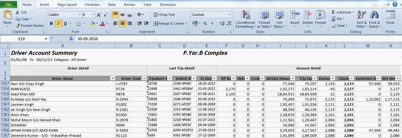
If above excel sheet. I have maintained ledger balance of Drivers of my company. This file has 2855 Rows (your file might have more or less).

While I have to view other records, I have to scroll the page. This will look like this snapshot.

What data is in column F, or G or H. If I do not remember, we have to scroll back and view headers and then come back to last position. To overcome this problem, Microsoft Excel has built-in feature called Freeze Rows or Panes. In this post, we will learn how to fix a Top row or more rows at same time.
If you are using Excel 2007, 2010 and 2013 the method is similar.

Lets go to process.

1. If Top row of your sheet is header, you need not to do anything, But if you have headers in second or third row, Select entire row below from header row by clicking in Row name..
2. Click on View Tab on Office Ribbon.
3. Click on Freeze Top Row if header in First row or Freeze Panes if header in second or third row. 

Now look at this. How it looked after scrolling down.

One thing most important about this feature. Your settings are saved within file. Means if you share file with other via email or other sharing tools, your settings remains same even if Microsoft Office version changes or system varies.

All the Best. If you found if helpful, do not forget to post a thank or +1 on Google.
+John Bhatt 

Read More